

The Rachford–Rice equation finds the vapor mole fraction of a two-phase mixture when the feed composition and equilibrium ratios are known. It is a compact way to solve the material-balance part of a flash calculation. It does not, on its own, supply the equilibrium ratios or prove phase stability.
For feed mole fractions z, equilibrium ratios K and vapor mole fraction beta, solve F(beta) = sum[z_i*(K_i-1)/(1+beta*(K_i-1))] = 0. Then calculate x_i = z_i/[1+beta*(K_i-1)] and y_i = K_i*x_i.
These relations follow from the component balances and K_i = y_i/x_i. See Penn State's analysis of flash objective functions for the mathematical framework.
Define a teaching case
Use the following synthetic input. A, B and C are abstract components; the K values are assumed for the exercise. The numbers are not a validated fluid model or a result from PvtLabOnline.
| Component | Feed mole fraction z | Assumed K |
|---|---|---|
| A | 0.50 | 2.00 |
| B | 0.30 | 0.75 |
| C | 0.20 | 0.20 |
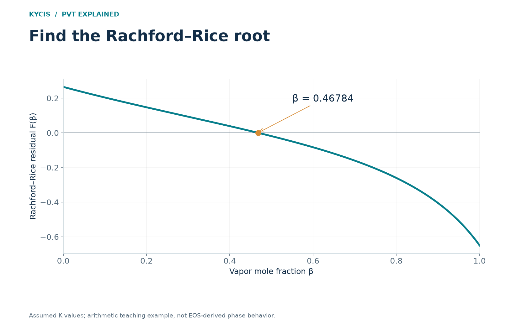
At beta = 0, the objective is 0.265. At beta = 1, it is -0.650. The sign change brackets a two-phase material-balance root between zero and one for these positive K values.
Solve within the bracket
A simple bisection procedure is sufficient for this example. Evaluate F at the midpoint of the bracket. Replace the endpoint having the same sign with that midpoint and repeat until the bracket is sufficiently small.
The result is beta = 0.4678409582, or approximately 46.7841 mol% vapor. Substitution gives:
| Component | Liquid mole fraction x | Vapor mole fraction y |
|---|---|---|
| A | 0.3406363593 | 0.6812727185 |
| B | 0.3397355515 | 0.2548016636 |
| C | 0.3196280892 | 0.0639256178 |
Both columns sum to approximately one. Reconstructing the feed with beta*y_i + (1-beta)*x_i recovers 0.50, 0.30 and 0.20. That independent substitution is a more informative check than simply observing that an iteration stopped.
Why the root is well behaved here
For positive K values and nonnegative feed fractions, the derivative is F'(beta) = -sum[z_i*(K_i-1)^2/(1+beta*(K_i-1))^2]. It is nonpositive wherever the expression is defined. With these nontrivial K values it is negative, so the objective decreases through the root.
On the physical interval from zero to one, positive K values keep the denominators positive. Bisection stays inside the initial bracket. A Newton step can be faster but should not be allowed to wander into an unphysical interval or cross a singularity.
Interpret a missing sign change carefully
If the endpoint values do not bracket an interior root, the assumed K values do not support a two-phase material-balance solution in that interval. This is useful information in a fixed-K exercise. In a real EOS calculation, it is not sufficient reason to declare that the original fluid must be single phase without considering the equilibrium and stability calculation.
Similarly, K values all close to one make phase compositions similar and the objective less informative. Near-critical calculations need more care than this deliberately simple exercise illustrates.
Connect the exercise to an online flash calculation
An engineering flash solver has additional work: select appropriate thermodynamic models, evaluate fugacity coefficients, update the phase compositions and determine the stable state. The hand calculation is best used to understand and audit a reported phase split, not as a replacement for those steps.
For the broader experimental context, see what laboratory PVT analysis measures. Contact KYCIS to discuss a PVT calculation question.
Endpoint tests and the near-critical limit
For positive fixed K values, F(0) = sum(z_i K_i) - 1 and F(1) = 1 - sum(z_i/K_i). With a nontrivial composition, an interior physical material-balance root requires F(0) > 0 and F(1) < 0. Equality at an endpoint is a limiting phase amount for those K values. If every active K equals one, F is zero for every beta: the equation cannot determine a unique phase fraction.
This explains why a tiny residual alone can be misleading. If K_i = 1 + epsilon_i, the magnitude of the derivative is approximately sum(z_i epsilon_i²) when the epsilon values are small. A nearly flat objective can give a small residual over a wide range of beta. Check the bracket width and phase compositions, not just F.
The outer EOS problem still has to be solved
Rachford–Rice solves phase amounts for supplied K values. An EOS algorithm must also update fugacity coefficients and examine stability; blindly clipping a negative-flash root into [0,1] does not perform those tasks. Modern implementations combine several numerical strategies, as illustrated by NeqSim’s TP-flash algorithm documentation. This is an algorithm reference, not a claim that PvtLabOnline uses NeqSim.
Use a PvtLabOnline two-phase result as an audit exercise: reconstruct component balances from the reported beta, x and y and compare positive-component fugacities where valid. Solver diagnostics unavailable in the interface cannot be inferred from a smooth plot.