
A PT flash calculation determines the equilibrium phase split of a fluid at a specified pressure, temperature and overall composition. Its most useful answers are the amount of vapor and liquid, the composition of each phase, and the properties of the phases that exist. Those answers make PT flash a useful starting point for learning PVT calculations and checking an individual operating condition.
The pressure and temperature are inputs. The calculation does not determine how much cooling, heating or pressure reduction a real piece of equipment requires to reach that condition. Keeping this distinction clear makes both the inputs and the results easier to interpret.
What goes into a PT flash calculation
Start with a composition whose basis is known. A table of mole percentages and a table of mass percentages describe different numerical inputs, even when both add to 100. Record the identities of the components as well as their amounts. A measured C7+ fraction needs a model representation; it cannot simply be treated as pure normal heptane.
Next specify absolute pressure, temperature and the fluid model. The model includes the equation of state, component properties, mixing assumptions and any heavy fraction characterization. A calculation labeled Peng–Robinson is not fully specified until those choices are known.
For hydrocarbon vapor–liquid equilibrium, the solver combines component balances with equilibrium conditions. The familiar Rachford–Rice equation is part of this framework when equilibrium ratios are available. An EOS flash also has to determine consistent ratios and establish the applicable phase state. Penn State's flash calculation notes explain the relationship between the ratios and the phase split.
A worked balance you can check by hand
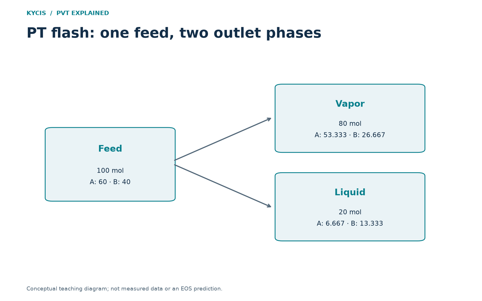
Consider a fictional two-component mixture. The following numbers are an arithmetic teaching example, not laboratory data or a validated EOS prediction. Components A and B have feed mole fractions 0.60 and 0.40. Suppose a reported calculation gives a vapor mole fraction of 0.80 and these phase compositions:
| Component | Feed z | Liquid x | Vapor y |
|---|---|---|---|
| A | 0.600000 | 0.333333 | 0.666667 |
| B | 0.400000 | 0.666667 | 0.333333 |
On a basis of 100 mol of feed, there are 80 mol of vapor and 20 mol of liquid. Component A contributes approximately 53.333 mol in the vapor and 6.667 mol in the liquid. Their sum is 60 mol, agreeing with the feed. Component B contributes 26.667 mol in the vapor and 13.333 mol in the liquid, totaling 40 mol.
The general check is z_i = beta*y_i + (1-beta)*x_i, where beta is vapor mole fraction. Both phase composition columns should also sum to one. Small differences from rounded display values are expected; substantial differences deserve investigation.
This example demonstrates material balance only. Without a temperature, pressure and thermodynamic model, it does not establish that these phases are at equilibrium. A successful balance is necessary, but it cannot validate an EOS prediction by itself.
Read the phase fraction before the property table
If the result is a stable single phase, properties of an absent phase should not be interpreted as a real product stream. A blank liquid density in a vapor-only state is not a liquid density of zero. Likewise, a vapor mole fraction of 0.80 does not mean that 80% of the mass or 80% of the volume is vapor.
Check the phase compositions next. Their enrichment patterns explain why feed, liquid and vapor molecular weights differ. Only then compare density, compressibility factor or other available properties, keeping the phase and basis attached to each value.
Turn one flash into a useful comparison
Choose a specific question, such as how the phase split changes over a short pressure range at fixed temperature. Keep the feed and model unchanged, calculate the selected conditions, and compare both the phase fraction and phase compositions. Add conditions near any transition rather than drawing a conclusion from one isolated point.
Several calculations on the same feed are independent equilibrium states. They do not automatically represent successive separator stages, because a real downstream stage receives the material passed to it by the upstream stage.
For the broader experimental context, see what laboratory PVT analysis measures. Contact KYCIS to discuss a PVT calculation question.
Application: screen a cooler outlet for hydrocarbon liquid
Suppose the question is whether a defined gas feed forms hydrocarbon liquid over its expected cooler-outlet temperature range. Obtain the actual outlet pressure range and composition first. Select a warm point, the intended normal outlet and a colder credible condition. These are independent PT states of the same feed; the study does not determine cooler duty.
- Calculate the phase envelope for the selected composition and EOS to locate the relevant boundary.
- Evaluate the chosen outlet PT pairs. If phase presence changes, add closer points within that interval. A coarse scan can miss a narrow two-phase region.
- Record liquid mass fraction, liquid density and phase composition wherever valid. Report a failed point separately from a vapor-only point.
- Translate equilibrium fraction to an amount using the actual feed basis, then decide which conditions need a more detailed equipment study.
For an arithmetic illustration, a 1,000 kg/h feed with a hypothetical equilibrium liquid mass fraction of 0.015 contains 15 kg/h of liquid. At an assumed liquid density of 600 kg/m³, its equilibrium liquid volume rate is 0.025 m³/h at that state. These are conversions, not PvtLabOnline predictions or separator carryover rates.
PvtLabOnline’s development workflow accepts up to ten independent PT pairs in a result set and displays phase amounts and applicable phase properties. That supports this focused screening task. Preserve the first set before refining it, because a new run replaces the module’s working result.