1. The latency budget in a SCADA feedback loop
Most pipeline-grade SCADA systems run on a 1 Hz polling cycle: every second, the historian writes a fresh row of measurements from gas chromatographs, pressure transmitters, temperature probes, and flow meters. Inside that 1-second budget the control system has to do a lot — read each meter, validate the values, push them to the historian, evaluate alarm and interlock logic, and, increasingly, run derived calculations like hydrocarbon dew point (HCDP), water dew point, and phase envelope.
Some of that work is fast and predictable. Reading a Modbus register or pushing a value to a real-time database takes milliseconds. Other work is variable and can blow the budget if it’s poorly bounded. Dew-point calculation lives in the second category. It depends on the gas composition, the operating point, and the underlying equation of state (EOS), and a careless implementation can spend hundreds of milliseconds or even multiple seconds per call when the operating point is near critical or the EOS solver struggles to converge.
If a single dew-point call can sit at 800 ms on a bad input, you have no business calling it from the 1-second polling loop. You either delay your other alarm logic, queue the calls, or fall back to running them out of band and getting stale values back into the control system on a 30-second or minute cadence — which is exactly the integration pattern we have seen most pipeline operators settle for historically. That is not because they did not want real-time dew point; it is because the latency story did not support it.
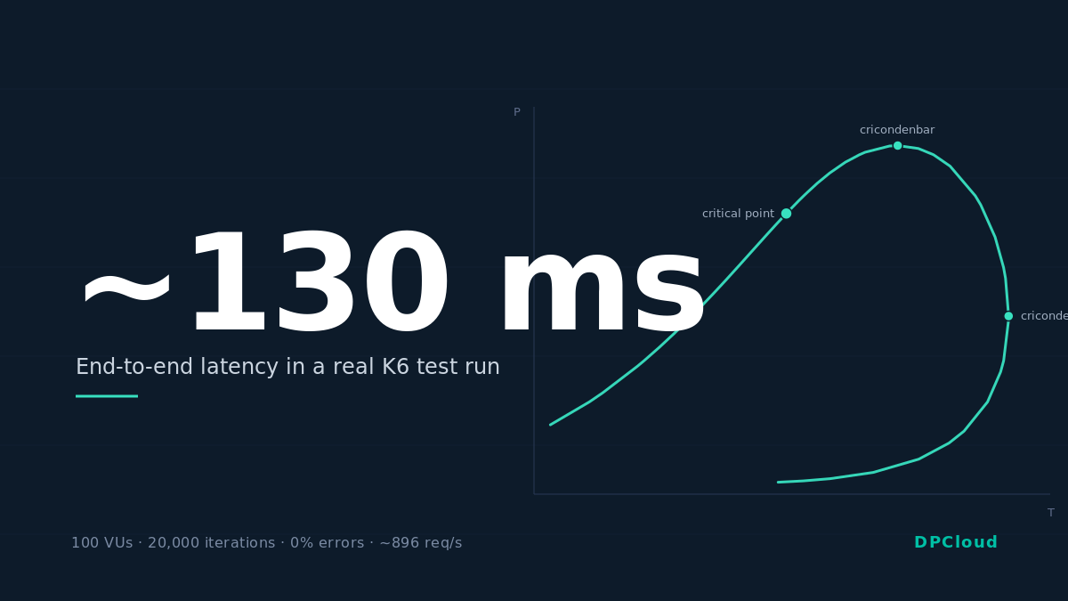
DPCloud’s design target was to bring dew-point and phase-envelope calls back into the inner SCADA loop. To make that practical, the round-trip latency a SCADA host actually experiences needs to leave clear margin within the per-cycle budget, and the long-tail latency needs to be bounded enough that one slow call does not cascade into a missed cycle. The headline number we publish — approximately 130 ms round trip — is the conservative bound that came out of load testing under representative concurrency. The rest of this article is about how the calculation engine and the deployment architecture combine to make that bound stable.
For the integration patterns this latency target unlocks on the SCADA side, see our earlier piece on integrating real-time dew point calculations into your SCADA system.
2. What “130 ms” actually measures
The headline latency number for DPCloud is approximately 130 ms round trip, measured from a client outside the data center. That phrasing matters. It is not the CPU time spent inside the dew-point solver; it is the elapsed time a SCADA host calling the REST endpoint from a typical industrial network waits before the response comes back.
In representative tests on a 24-component natural-gas mixture, the server-side calculation itself is in the single-digit to low-double-digit millisecond range, typically about 5 to 15 ms. The exact number depends on whether the request reaches a warm container, how close the operating point is to the cricondentherm, and how many stability checks the solver needs to run. The rest of the observed round trip is network latency, connection/TLS overhead amortized across requests, and load-balancer or gateway hops.
We report the slower end-to-end number rather than the faster server-only number deliberately. In real deployments, the network leg is what the SCADA polling loop actually experiences. For a 1 Hz dew-point feedback loop, that distinction matters more than the raw solver timing — what determines feasibility is the round trip your control system actually waits on, not the time the engine takes in isolation.
A second point worth being explicit about: the 130 ms figure refers to the conservative end of a healthy distribution rather than the median. In our K6 load tests, the median round trip to the hydrocarbon dew-point endpoint sat around 86 ms; the 90th percentile was 131 ms; the 95th was 166 ms. We picked 130 ms as the public bound because it covers the great majority of calls under representative concurrency and leaves visible headroom against the SCADA cycle, not because the typical call needs that long.
Section 8 expands on the full latency distribution and what dominates the variance.
3. Why phase-envelope continuation, not point-by-point flash
The single biggest engineering choice in DPCloud’s performance budget is not a low-level optimization; it is a high-level algorithmic one. We do not compute the phase envelope by running an independent flash calculation at every pressure-temperature point on a grid. We use phase-envelope continuation.
The naïve approach is straightforward to explain. You sweep a pressure-temperature plane, you pick a discretization (say, every 0.5 bar and every 0.5 K), and at each grid point you ask the EOS: is this a single phase or two phases, and if two, what is the phase split? Inside each call the solver iterates from a fresh initial guess until it converges. To trace out a phase envelope you have to do this hundreds or thousands of times across the plane. The math is correct. It just wastes most of the work.
Continuation methods exploit the structure of the problem to avoid that waste. The phase envelope is a smooth one-dimensional curve in PT space, with a few exceptions near the critical point that need explicit handling. If you find one valid point on the envelope, the next point a small step away is, by definition, close in both pressure and temperature, and the K-values describing the phase split do not change discontinuously between them. A predictor step uses the local tangent of the envelope to predict where the next valid point should be; a corrector step refines that prediction back onto the envelope itself.
In practice this means tracing out an entire phase envelope with on the order of tens of well-placed points rather than hundreds of grid-aligned flashes. The continuation algorithm starts at a known anchor — often the bubble point at low pressure — takes a tangent step, applies a Newton-based corrector to land back on the envelope, repeats, and stops at the second anchor (the critical point or a user-specified pressure ceiling). Along the way it picks up the cricondentherm and cricondenbar as named features rather than as accidents of grid resolution.
This algorithmic choice is the difference between a phase-envelope endpoint that finishes in around 100 milliseconds and one that takes seconds. The lower-level optimizations described in the next sections matter, but they sit on top of this foundation.
4. Newton-type corrector and bracketed bisection dew-point root-finding
Continuation is not enough on its own — the corrector step that pulls each predicted point back onto the envelope still has to converge. DPCloud uses a Newton-type corrector for that step. Newton’s method is quadratically convergent when it converges, and from a predicted point that is already close to the envelope it usually does, in three to six iterations.
But “usually” is not a guarantee, and a real-time engine that calls into a SCADA loop has to handle the cases where Newton would misbehave. Two specific situations matter. One is when the predicted point is so close to a turning point of the envelope that the Jacobian becomes ill-conditioned. The other is the dew-point calculation when it is invoked as a one-off — not as part of a continuation walk, but as a direct API call from the SCADA host asking what is the HCDP at this composition, this pressure, right now?
For the standalone dew-point case we do not rely on Newton with an initial guess. We use a bracketed bisection root-finder. Bisection is slower than Newton in the convergent regime — typically dozens of iterations versus a handful — but each iteration is cheap, and bisection has the property that once you have a valid bracket (a pressure or temperature pair that brackets a sign change in the dew-point residual) it cannot diverge. For a 1 Hz SCADA loop, “always converges in a bounded number of iterations” is more valuable than “converges quickly when it does.” The runtime cost of bracketed bisection at single-digit milliseconds is well inside the latency budget; the cost of a Newton solver that occasionally fails and needs a restart is not.
The result is an engine where the fast path for envelope tracing uses Newton because Newton is fast where Newton works, and the safe path for standalone dew-point queries uses bisection because bisection works everywhere. Both paths land at the same answer.
5. Stability analysis with TPD and Hebden-type trust-region minimization
Continuation alone does not tell you whether you are inside or outside the two-phase region. For that the EOS solver needs a stability test, and the standard tool is the Tangent Plane Distance (TPD) criterion.
The idea behind TPD is geometric. If a candidate trial-phase composition reduces the system’s total Gibbs free energy below the single-phase value, the single-phase assumption was wrong and the system will split. The TPD function is the difference. A negative TPD anywhere in composition space means instability; a non-negative TPD everywhere means the single phase is the stable solution. So the stability test reduces to a global minimization problem: find the minimum of TPD over composition space and check its sign.
Where this gets hard is near the critical region, near the cricondentherm, and at compositions with strongly non-ideal interactions. Unconstrained Newton-style minimization on TPD can step outside the physical region (negative mole fractions), oscillate between local minima, or simply diverge. The classical solution is to use a trust-region method that wraps Newton steps in a controlled radius and refuses any step that increases the objective.
DPCloud uses a Hebden-type trust-region minimization for TPD. Hebden’s original 1973 formulation gives an explicit way to compute a trust-region-constrained Newton step: solve a parameterized linear system that interpolates between a pure Newton step (when the trust region is large) and a pure gradient-descent step (when the trust region is small), with the parameter chosen so the step length lands exactly on the boundary of the trust region. The practical effect is that the minimizer never takes a wild step into a region where the EOS evaluation is unreliable, and it also does not slow down to gradient-descent pace when Newton would do fine.
This matters for runtime in two ways. First, the worst-case iteration count is bounded, which keeps the latency tail under control. Second, in well-behaved regions the trust-region constraint barely activates and the iteration cost stays close to the pure-Newton number.
6. Adaptive step size along the envelope
The last algorithmic ingredient is adaptive step size control along the continuation walk. The predictor does not take a fixed step in pressure or temperature; it takes a step in arc length along the envelope curve, and the size of that step is adjusted at each iteration based on the local curvature and on how hard the corrector had to work on the previous step.
In the straight, well-behaved sections of an envelope — say, the bubble-point side at low pressure for a typical pipeline gas — the steps can be large, and the corrector converges in a couple of Newton iterations each. As the walk approaches the cricondentherm or cricondenbar, the local curvature spikes, the Jacobian conditioning degrades, and the corrector starts working harder. The adaptive step controller responds by shrinking the next step until the corrector is comfortable again. After the turning point, as the curve straightens out, the step size grows back.
The benefit is not raw speed; it is the opposite. The adaptive controller is what lets the algorithm spend its computational budget where the geometry actually demands it. A fixed-step continuation either wastes work in the straight sections or breaks in the turning sections. The adaptive version stays cheap in the easy regions and slows down only where it has to.
7. What we deliberately did NOT do
Listing the optimizations we adopted is half the picture. The other half is the simplifications we considered and rejected, because each of them would have saved time at the cost of accuracy or robustness that the use case cannot afford.
No cross-call K-value warm-start. In a sequential series of pipeline dew-point calls, you might be tempted to cache the converged K-values from one call and feed them as the initial guess for the next. The intuition is that operating points evolve slowly. The intuition is also wrong in practice: gas composition can change discontinuously between scan cycles — a new GC analysis result arrives, the upstream blend changes, an operator switches sources. A warm-start that ignores that discontinuity can converge to the wrong basin and silently return the wrong answer. We picked correctness over the few milliseconds of cold-start cost.
No precomputed envelope interpolation. It is common to precompute an envelope for a representative gas composition and serve subsequent queries by interpolating against the stored curve. This is fast and very nearly accurate enough — except that the precomputed envelope’s cricondentherm and cricondenbar are tied to a fixed composition, and the moment the upstream gas composition shifts, those critical points move and an interpolated answer is wrong in a way that matters. We compute the envelope fresh every time.
No parallel TPD evaluation. TPD minimization with multiple trial-phase compositions is a candidate for parallelism on paper. In practice, at the problem size involved — 24 components, a handful of trial seeds, single-millisecond per evaluation — thread-pool dispatch overhead eats the speedup, and the result is variance in latency rather than a faster median. We run the trial phases sequentially and use the bounded iteration count of the Hebden-type trust region to keep the tail in check.
No EOS substitution. Some implementations switch to Soave-Redlich-Kwong (SRK) or even an ideal-gas approximation at “easy” operating points to save a few milliseconds. We stay on Peng-Robinson everywhere. The accuracy difference between PR and SRK at typical pipeline conditions is small enough that customers would not notice in a benchmark, and large enough at certain custody-transfer and cricondentherm conditions to matter for alarm-margin calculations. We do not want the answer to depend on which code path the request happened to take.
8. Latency distribution in K6 load testing
The latency numbers in this article come from a K6 stress test against the production deployment of DPCloud, running 100 concurrent virtual users hitting three endpoints — hydrocarbon dew point, water dew point, and full phase envelope — for 20,000 total iterations. Under this specific test profile, aggregate throughput on a single deployment was approximately 896 requests per second. Every one of the 40,000 response-validation checks succeeded; the failure rate over the test was 0%.
The distribution by endpoint (round-trip time in milliseconds, measured from the K6 client outside the data center):
| Endpoint | median | p90 | p95 | p99 |
|---|---|---|---|---|
| Hydrocarbon dew point | 86 | 131 | 166 | 333 |
| Water dew point | 84 | 123 | 151 | 340 |
| Phase envelope | 92 | 140 | 183 | 331 |
A few observations about the shape of the distribution.
First, the median is well below 100 ms across all three endpoints. Phase-envelope calculations, which do the most work, are about ten percent slower at the median than single-point dew-point calls but not dramatically so — the continuation method scales gracefully with the complexity of the envelope shape.
Second, the gap between p90 and p99 is largely network-driven, not solver-driven. The K6 HTTP-phase breakdown shows connection and TLS-handshake costs amortized across reused connections to near zero, but per-request “waiting time” (the server’s time-to-first-byte from the client’s perspective) tracks closely with the overall round-trip distribution. That tells us most of the tail latency rides on the network path, not on the solver.
Third, the worst outlier in this run was a single tail event during the test window. We track such events across runs, but it is not representative of the normal latency profile; the solver itself remains bounded in iteration count.
For a deeper view of how this latency profile compares with legacy desktop EOS software typically used for the same calculations, see Comparing Dew Point Calculation Software: Legacy Systems vs. Modern API Approach.
9. Talk to engineering
If you are considering DPCloud for a real-time SCADA dew-point or phase-envelope integration, the fastest way to see the latency story in your own environment is to run the live demo against your own representative gas composition — it makes the same engine calls described in this article.
For an integration scoping conversation, or to discuss on-premise / air-gapped deployments where the network leg is replaced by your internal network, email api@kycis.com or use the contact page.
Related: Dew Point Measurement vs Real-Time Calculation: ISO 18453, Chilled Mirrors, and When to Trust Which — A practical framework for when to trust certified measurement vs real-time calculation in pipeline gas-quality decisions.