
A bubble point is a saturated-liquid boundary where the equilibrium vapor fraction approaches zero. A dew point is a saturated-vapor boundary where the equilibrium liquid fraction approaches zero. Whether crossing that boundary creates or removes a phase depends on the operating path and its direction. For a mixture, each calculation needs a composition and one specified state variable: pressure for a temperature calculation, or temperature for a pressure calculation.
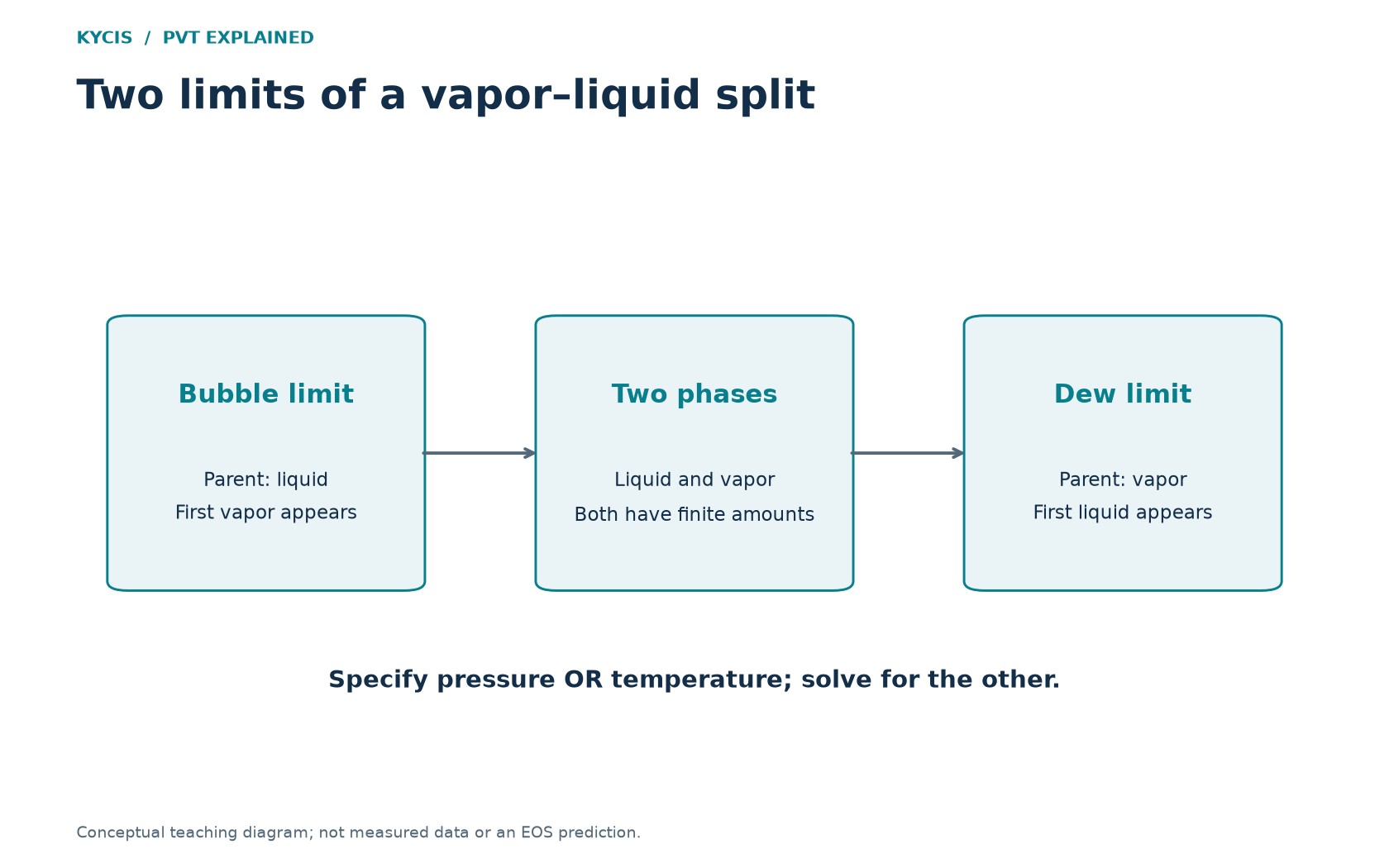
This gives four different questions. Confusing them can produce apparently contradictory numbers from otherwise consistent calculations.
Specify the question completely
| Calculation | Given | Solved |
|---|---|---|
| Bubble temperature | Liquid composition and pressure | Temperature at vapor onset |
| Dew temperature | Vapor composition and pressure | Temperature at liquid onset |
| Bubble pressure | Liquid composition and temperature | Pressure at vapor onset |
| Dew pressure | Vapor composition and temperature | Pressure at liquid onset |
At the boundary, the incipient phase has essentially zero amount, but it has a limiting composition. That composition generally differs from the composition of the phase already present. Away from the boundary, PT flash determines finite amounts and compositions of both phases.
The IDAES bubble and dew point documentation distinguishes these formulations and the equilibrium equations involved. A temperature from one formulation should not be compared directly with a pressure from another.
What is each bubble or dew calculation used for?
Choose the calculation from the quantity you control and the phase change you need to locate. The examples below describe the relevant operating branch; retrograde behavior can change the direction of phase appearance.
| Calculation | Practical question | Typical uses |
|---|---|---|
| Bubble-point pressure at a given temperature | How far can this liquid be depressurized before free vapor first appears? | Locating gas liberation during oil depletion; screening liquid sampling, transfer and depressurization conditions; choosing pressure points for an oil PVT study. |
| Dew-point pressure at a given temperature | Which pressure boundary does this gas cross before a liquid phase appears or disappears? | Assessing condensate onset during gas-condensate pressure decline; checking gas-processing pressure paths. Specify the upper or lower dew branch where two roots exist. |
| Bubble-point temperature at a given pressure | At this pressure, where does a heated liquid begin to form vapor on the selected branch? | Screening liquid-feed preheating and boiling onset; choosing conditions for a flash or vaporization study. |
| Dew-point temperature at a given pressure | At this pressure, where does a cooling gas begin to form liquid on the selected branch? | Hydrocarbon dew-point assessment; identifying possible condensation in coolers and heat exchangers; choosing gas-cooling or condensation conditions. |
A saturation boundary locates the onset, not the amount of liquid or vapor formed. It does not by itself size a separator or heat exchanger, establish a safe operating margin, or predict a production rate. Hydrocarbon and water dew points also require different component and phase descriptions.
Use K values to understand the limits
Define an equilibrium ratio as K_i = y_i/x_i, where y and x are vapor and liquid mole fractions. At a bubble point the feed is almost entirely liquid, so x approaches the overall composition z. The limiting relation is sum(z_i*K_i) = 1. At a dew point y approaches z, giving sum(z_i/K_i) = 1.
These relations are useful checks, but real-mixture K values are not fixed universal constants. They depend on the state and phase compositions. A consistent EOS calculation must determine them together with the boundary state.
An arithmetic example of the two limits
Assume a fictional binary mixture has K values 2.0 and 0.5 at a stated but otherwise unspecified condition. A bubble-point liquid composition of one-third A and two-thirds B satisfies the first relation: (1/3)*2 + (2/3)*0.5 = 1. Its incipient vapor contains two-thirds A and one-third B.
A dew-point vapor with two-thirds A and one-third B satisfies the second relation: (2/3)/2 + (1/3)/0.5 = 1. Its incipient liquid has the original one-third/two-thirds composition.
This is a consistency example using assumed K values. It does not calculate a bubble or dew temperature for any real fluid. A numerical pressure or temperature would require additional thermodynamic information.
Retrograde behavior: why a boundary calculation can have two answers
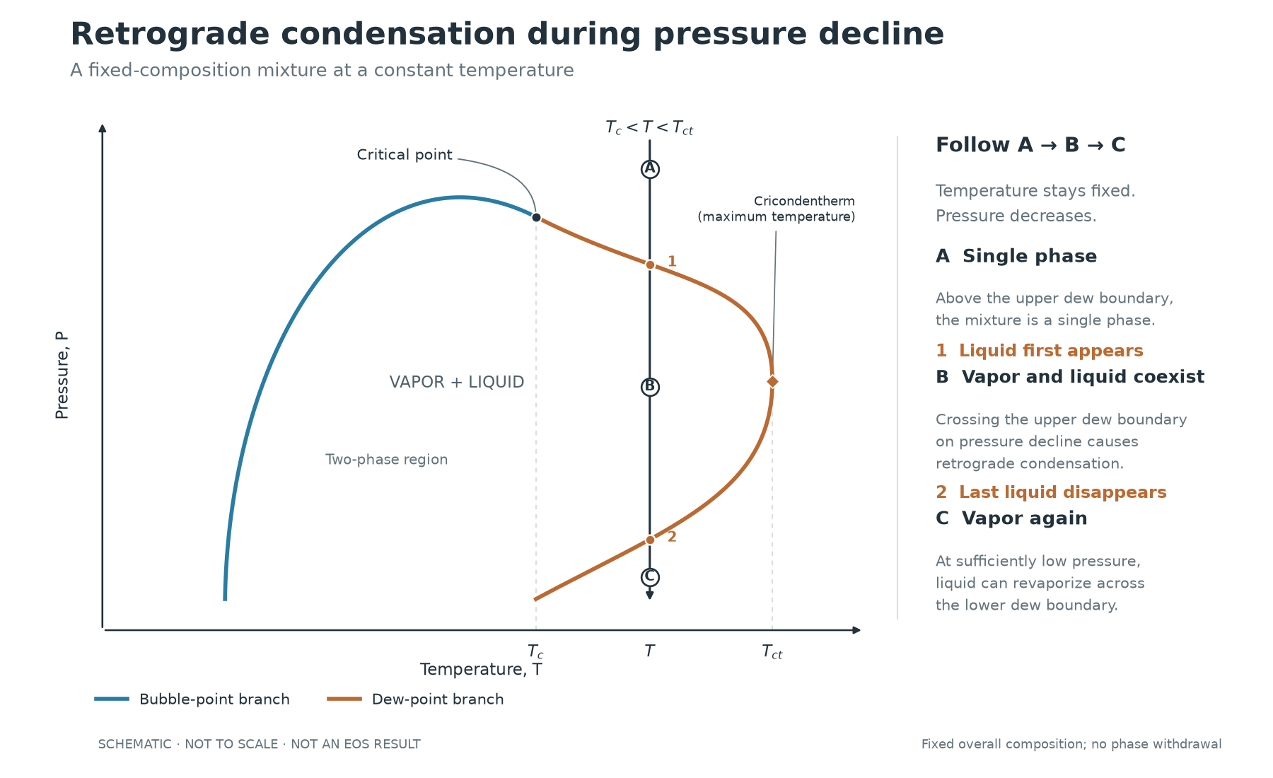
For a fixed overall composition, a conventional gas-condensate envelope can have two dew-point pressures at the same temperature when the temperature lies between the mixture critical temperature, Tc, and the cricondentherm, Tct. Starting above the upper dew pressure and reducing pressure at constant temperature can produce liquid. This is retrograde condensation: liquid forms during isothermal pressure decline, contrary to the usual tendency for expansion to favor vaporization.
Along this fixed-composition equilibrium path, the liquid fraction can rise to a maximum and then fall. If the path continues far enough, the last liquid disappears at the lower dew pressure. Both intersections are dew points because the equilibrium liquid fraction approaches zero at each boundary. The lower intersection may be outside the practical operating range. See the Penn State explanation of retrograde behavior.
What are the upper and lower dew pressures useful for?
The upper dew pressure identifies condensate onset on this isothermal pressure-decline path. It helps choose pressure intervals for gas-condensate PVT analysis and the nearby flash conditions at which liquid formation needs to be assessed. A boundary alone does not quantify condensate loss or flow impairment.
The lower dew pressure identifies where the last liquid vanishes in the same fixed-composition model. It helps check whether the full envelope has been traced and whether a saturation solver found the intended root. It is not a promise that a producing reservoir will return to a single gas phase at that pressure: withdrawal and phase retention can change the remaining composition.
Temperature sweeps can also have multiple boundaries
For a conventional envelope, a constant-pressure line between the critical pressure and the cricondenbar can intersect two bubble-point temperatures. Near the higher-temperature boundary, further heating can reduce the vapor fraction until it disappears into a single liquid-like phase. Reversing that segment can generate vapor by cooling. These are bubble roots, not the two dew pressures illustrated above. The NBS review of phase equilibria describes this type of retrograde loop.
How to select the relevant root
- Specify the overall composition, EOS, fixed variable and direction of travel.
- Trace the phase envelope to identify the relevant pressure or temperature branch.
- Run stable PT flashes on both sides of a candidate boundary to distinguish phase appearance from disappearance.
- Report the selected branch and whether phase fractions are on a mole, mass or volume basis.
NIST REFPROP documentation notes the difficulty of finding a second root in the retrograde region. Numerical convergence alone does not establish that a solver found the boundary relevant to your process.
This fixed-composition scan is not a constant-volume-depletion experiment or a reservoir production forecast. A CVD experiment withdraws fluid between stages, changing the overall composition remaining in the cell.
Avoid three common comparison errors
First, keep the sample composition consistent. A dew pressure for separated gas need not match a boundary calculated for the overall feed.
Second, record the pressure basis. A temperature measured at a stated gauge pressure must be compared with a calculation at the corresponding absolute pressure.
Third, distinguish a boundary at a selected pressure from an extremum of the entire phase envelope. A cricondentherm is not a replacement for the dew temperature at every operating pressure.
When is another PVT calculation more useful?
- Phase envelope: use it when the operating path spans a range of pressures and temperatures, when you need to distinguish branches or multiple roots, or when critical conditions and envelope extremes matter. The boundary alone does not give the finite liquid amount inside the envelope.
- PT flash: use it when pressure, temperature and overall composition are known and you need the equilibrium phase state, phase fractions and phase compositions. It can assess liquid dropout at selected conditions and provide an equilibrium building block for separation studies; one flash does not simulate an entire depletion experiment or process.
- Heavy-fraction characterization: use it when a C7+ or another unresolved fraction must be represented by pseudocomponents before an EOS calculation. It supplies a model description from the available analytical and bulk-property data; it does not replace measurements or automatically validate the resulting fluid model.
For example, a gas-condensate study may first characterize an unresolved heavy fraction, trace the phase envelope, select the upper dew-pressure crossing on a fixed-composition isothermal path, and then run PT flashes below that boundary to examine the predicted phase split. The PVT calculations guide connects these tasks.
Use a boundary to choose flash conditions
Once the boundary is understood, select PT points on the operating path and inspect the predicted phase fractions. This turns an onset calculation into a more useful description of the states around it. The size of the step should be chosen for the question and the numerical resolution, not copied as a universal temperature or pressure margin.
PvtLabOnline is available for completely free browser-based phase-envelope and PT-flash calculations, with characterization when the composition requires it. Create an account and verify your email to use the calculation workspace. Review the public PVT calculations guide, then open the online calculator. The hydrocarbon and water dew point guide explains a separate distinction that also matters when interpreting a dew-point result.
Connect the boundary definition to a calculation
With consistent equilibrium ratios, a bubble boundary satisfies sum(x_i K_i) = 1 as vapor amount approaches zero; a dew boundary satisfies sum(y_i/K_i) = 1 as liquid amount approaches zero. In an EOS calculation the K values depend on the trial phase compositions, so these expressions are not independent closed-form answers. A near-unity K solution also requires care in the critical region.
For an oil pressure check at fixed temperature, compare the operating pressure with the relevant bubble pressure, then use PT flash below the boundary to quantify gas liberation for the specified composition. For gas cooling at fixed pressure, compare temperature with the dew-temperature crossing, then quantify the condensed amount. For retrograde gas-condensate behavior, record which dew-pressure branch is crossed and the direction of travel.
PvtLabOnline’s verified modules provide envelope and PT calculations for these focused checks; this article’s four saturation questions should not be read as a claim that four separate bubble/dew solver screens are available. Inspect the calculated curve and nearby PT results, with adequate resolution, before reporting a boundary for a real operating decision.